Deep learning notes from siraj on youtube
1. Make a Prediction
- Data parsing and processing using data frames
- Splitting our data into a training and testing set
- Simple linear regression modal to find our line of best fit
- Slope formula - \(y = mx + b\)
Introduction
What is deep learning?
A neural network is a machine learning model, when we create neural networks that are many layers deep, that’s Deep Learning.
Deep learning is a subset of machine learning that’s outperformed every other type of model.
Task
- This task uses a supervised approach (with labelled data)
- The type of machine learning task we’ll perform is called regression.
Create a new virtualenv and switch to it.
# create a new virtual environment
mkvirtualenv deeplearning

# switch to it
workon deeplearning

# install dependencies - we must use version 1 of matplotlib
pip install -U numpy pandas scikit-learn scipy 'matplotlib==1.5.1'
| Brain | Body |
|---|---|
| 3.385 | 44.500 |
| 0.480 | 15.500 |
| 1.350 | 8.100 |
| 465.000 | 423.000 |
Here’s my jupyter notebook for this lesson.
import warnings
warnings.filterwarnings(action="ignore", module="scipy", message="^internal gelsd")
import pandas as pd
from sklearn import linear_model
import matplotlib.pyplot as plt

%matplotlib inline

# Read our data into a pandas data-frame object
# which is a 2d data structure of rows and columns
dataframe = pd.read_fwf('brain_body.txt')
x_values = dataframe[['Brain']]
y_values = dataframe[['Body']]

# linear regression helps find the relationship between our 2 vars to find the only line of best fit
# Use scikits linear_model object to init our linear regression model
body_reg = linear_model.LinearRegression()

# Fit our model on our x,y value pairs
body_reg.fit(x_values, y_values)

# Now we have the line of best fit, we can plot it on a graph

# Scatter plot
plt.scatter(x_values, y_values)

# Plot our regression line
# "for ever x value we have, predict the associated y value
#  and draw a line that intersects all those points"
plt.plot(x_values, body_reg.predict(x_values))

# Save it to a file
# plt.savefig('best-fit.png', bbox_inches='tight')

# Show it
plt.show()
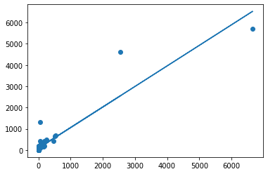
The x axis represents brain weights.
The y axis represents body weights.
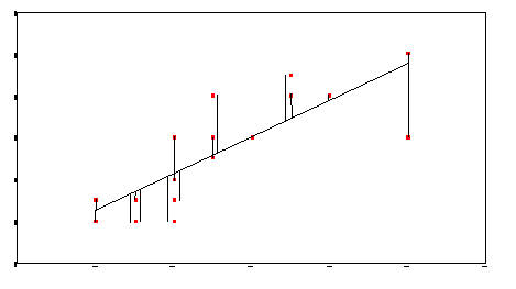
Challenge dataset
import pandas as pd
from sklearn import linear_model
import matplotlib.pyplot as plt
import numpy as np
import warnings
warnings.filterwarnings(action="ignore", module="scipy", message="^internal gelsd")
from IPython.display import display
Data cleaning
Our data is in a different format, we don't have heading columns, so we need to clean it up.
We also split our data into a training and testing set.
global df

# Read our data into a pandas data-frame object
df = pd.read_csv('challenge.csv', names=['X', 'Y'])

# Split our data into a test and training set (so we can calculate the error)
# http://scikit-learn.org/stable/modules/generated/sklearn.model_selection.train_test_split.html
from sklearn.model_selection import train_test_split
X_train, X_test, y_train, y_test = np.asarray(train_test_split(df['X'], df['Y'], test_size=0.1))

"Dataframe length: %s, X_train: %s, X_test: %s, y_train: %s, y_test: %s" % (len(df), len(X_train), len(X_test), len(y_train), len(y_test))
X_train, X_test, y_train, y_test are all of type pandas.core.series.Series.
Series is a one-dimensional labeled array capable of holding any data type (integers, strings, floating point numbers, Python objects, etc.). The axis labels are collectively referred to as the index.
Create our model
Create a LinearRegression model and fit our line.
We need to reshape our training data from (87,) to (87,1)
# (87,)
[1,2,3,86,87]

# (87,1)
[[1],[2],[3],[86],[87]]

# np.array([1,2,3,86,87]).shape           # (5,)
# np.array([[1],[2],[3],[86],[87]]).shape # (5,1)
http://cs231n.github.io/python-numpy-tutorial/#array-indexing
# linear regression helps find the relationship between our 2 vars to find the only line of best fit
# Use scikits linear_model object to init our linear regression model
reg = linear_model.LinearRegression()

# Fit our model on our x,y value pairs
# https://docs.scipy.org/doc/numpy-1.13.0/reference/generated/numpy.reshape.html
x = reg.fit(X_train.values.reshape(-1, 1), y_train.values.reshape(-1, 1))

# Returns the mean accuracy on the given test data and labels.
score = reg.score(X_test.values.reshape(-1, 1), y_test.values.reshape(-1, 1))

score
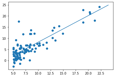
# Now we have the line of best fit, we can plot it on a graph

# Create our horizontal axis ranging from 5-25
x_line = np.arange(5, 25).reshape(-1,1)

# Scatter plot
plt.scatter(df['X'], df['Y'])

# Plot our regression line
# "for ever x value we have, predict the associated y value
#  and draw a line that intersects all those points"
plt.plot(x_line, reg.predict(x_line))

# Show it
plt.show()
Slope formula example
Here's a simple example using a small dataset showing the slope formula.
$$y = mx + b$$This is a table of salary and years worked.
salary_data = {
    'year': [1,2,3,4,5,6,7,8,9,10],
    'salary': [40000,42000,43000,46000,48000,52000,58000,62000,65500,68000]
}
df = pd.DataFrame(data=salary_data)
df
# No train/test splitting as we only have 10 values
X_train = df['year'].values.reshape(-1, 1)
y_train = df['salary'].values.reshape(-1, 1)

# Create our linear model
reg = linear_model.LinearRegression()

# Fit our model on our x,y value pairs
x = reg.fit(X_train, y_train)

b = int(round(reg.intercept_[0]))
m = int(round(reg.coef_[0][0]))

"y = {}x + {}".format(m, b)
The above should show:
$$y = 3342x + 34067$$So if we were prediciting the salary for someone after 15 years, the formula would be.
$$y = (3342*15) + 34067$$$$y = 84197$$
2. Linear Regression using Gradient Descent
- Hyperparameters
- Sum of squared errors
- Local minima
- Gradient descent
- Partial derivative
Linear Regression with Gradient Descent
We use gradient descent to find the line of best fit in our data, which we can then use to make a prediction. The gradient is a direction of positive or negative which we update our current b and current m values with each time step until we find our local minima (lowest error).
Linear regression is plain machine learning, there is no neural network.
Linear regression using gradient descent is used everywhere in ML and DL, so it’s important to understand the core concept.
Linear regression is a linear approach for modeling the relationship between a scalar dependent variable y and one or more explanatory variables (or independent variables) denoted X.
The case of one explanatory variable is called simple linear regression. For more than one explanatory variable, the process is called multiple linear regression.
Hyperparameters
In the context of machine learning, hyperparameters are parameters whose values are set prior to the commencement of the learning process. By contrast, the values of other parameters are derived via training.
Examples of hyper-parameters include:
- Learning rate (can be dynamic)
- Number of hidden layers in a deep neural network
- Read more link
Local Minima
If we find the smallest error rate (our local minima), that’ll also give us the y-intercept and slope.
We can use these in our \(y=mx+b\) equation to get our line of best fit, which we can then use to make a prediction.
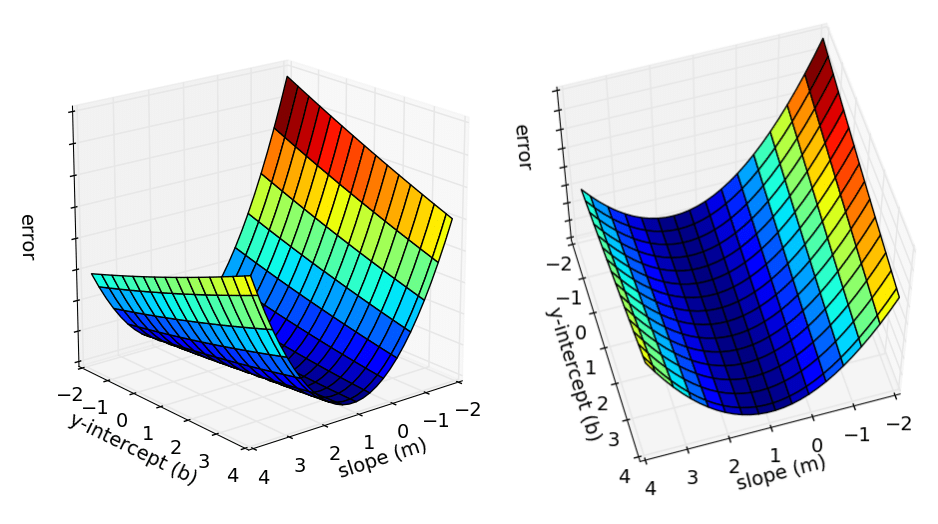
This graph shows 3 dimensions of all the possible values of the y intercept, the slope and error values.
We want to find the point where the error is smallest (our local minima). Looking at the graph, it’s the blue part at the bottom of the curve.
- Why local as oppose to non local?
- We have a simple graph with 1 local minima, sometimes you may have many minima, so you may want to find which minima (2nd order optimization).
- Do we always have 1 local minima?
- No, in complex cases there could be several local minima.
The gradient
https://www.youtube.com/watch?v=IHZwWFHWa-w
The way we get the smallest error, is by calculating the gradient.
The gradient gives us the direction to move the slope. It tells us to move positive (up) or negative (down), after completing our iterations, we should find our local minima - the point with the lowest errors.
If a function’s gradient can be computed using the partial derivative, it’s known as a differentiable function, and we can optimize it.
The gradient is a tangent line (a line that touches the function at one point only)
To calculate the gradient, we have compute the partial derivative with respect to our values b & m
Derivatives and partial derivatives
A derivative means the slope, let’s say we have the following function.
If \(a = 2\) then \(f(a) = 6\).
If we nudge \(a = 2.001\) then \(f(a) = 6.003\) moves 3 times as much.
So the slope (derivative) of \(f(a)\) at \(a = 2\) is \(3\).
The slope is defined as the \(\frac{height}{width}\) of the triangle, so in our example it would be \(\frac{0.003}{0.001} = 3\).
This is commonly written as \(\frac{d\;f(a)}{da} = 3\)
The formal definition of derivative says whenever you nudge a to the right by an infinitesimal amount (an infinitely tiny amount) if you do that does f(a) go up 3x as much as whatever was the tiny amount you nudged it by.
The partial derivative is when we change one variable and keep one variable constant to view the relationship between them.
Calculate the partial derivative of m:
Calculate the partial derivative of b:
Sum of squared errors
We want to compute the error/loss for the current time step (error/loss means the same thing), we use the sum of squared errors to do this.
Sum of squared errors example
given some points, measure the distance from each of those points to the line we have drawn and then square them, sum them all together and then divide by the total number of points
| Symbol | Description |
|---|---|
| \(\Sigma\) | Sigma notation - a set of values we are going to iterate over |
| \(\,i\,\) | Current index point in iteration |
| \(N\) | number of points |
| \(\,y\,\) | Current y point in our dataset |
| \(\frac 1N\) | Find the average of those |
| Measure the squared error values for all of N points | |
| The value returned is the sum of the squared errors - our error value | |
Measure the squared error values for all of N points.
The value returned is the sum of the squared errors - our error value.
We want to minimize this value every time step using gradient descent.
We have a \(y\) point from our dataset, and a \(y\) point on our line, we want to minimize the distance between both of those points.
We subtract the point in the dataset from the point on our line and then we square it to ensure the value is positive.
We don’t need the actual value, we only care about the magnitude of this value, we use it to minimize the error.
- We now have the difference between our “y intercepts”.
Further Reading
3. Make a neural network
- The McCulloch-Pitts Model of Neuron (1943)
- The Perceptron
- Forward propagation
- Backpropagate to update weights
Introduction
Let’s create our own neural network from scratch using just numpy.
The McCulloch-Pitts Model of Neuron (1943)

The McCulloch-Pitts Model of Neuron (1943)
- Take some binary inputs
- Sum them
- If the sum exceeds a threshold output a 0 or 1
The Perceptron by Frank Rosenblatt

The Perceptron by Frank Rosenblatt
Lesson #3 - Create a neural network
import numpy as np
from numpy import exp, array, random, dot
import matplotlib.pyplot as plt
from past.builtins import xrange
from IPython.display import display, Markdown
import numpy as np

# Custom logger to log one-line arrays
def logger(msg, log_array, nl=False):
    if not isinstance(log_array, np.ndarray):
        print('{message}'.format(message=msg))
    else:
        string_array = ', '.join(map(str, log_array))
        print('{message: <{fill}}: {array}'.format(message=msg, array=string_array, fill='35'))

    if nl is True:
        print('\n')
class NeuralNetwork():
    def __init__(self):
        # Seed the random generator so we get the same number each time
        np.random.seed(1)

        # We model a single neuron with 3 input connections 1 output connection
        # we assign random weights to a 3 x 1 matrix, with values in the range -1 to 1
        self.synaptic_weights = 2 * np.random.random((3,1)) -1
        display(Markdown('## Initializing Single Layer Feed Forward Network'))
        display(Markdown('Starting our network with the following random synaptic weights:'))
        display(Markdown('> ``%s``' % self.synaptic_weights))

    # The Sigmoid function, which describes an S shaped curve.
    # We pass the weighted sum of the inputs through this function to
    # normalise them between 0 and 1.
    # We can pass a np.array here to apply it to all values
    def __sigmoid(self, x):
        return 1 / (1 + np.exp(-x))

    # The derivative of the Sigmoid function.
    # This is the gradient of the Sigmoid curve. The slope.
    # It indicates how confident we are about the existing weight.
    def __sigmoid_derivative(self, x):
        return x * (1-x)

    # We train the neural network through a process of trial and error.
    # Adjusting the synaptic weights each time.
    def train(self, training_set_inputs, training_set_outputs, number_of_training_iterations):
        for iteration in xrange(number_of_training_iterations):
            if (iteration % 2000 == 0):
                logger('Iteration: %s' % iteration, False)
                logger('Current Synaptic Weights:', self.synaptic_weights)

            # Pass the training set through our neural network (a single neuron).
            output = self.predict(training_set_inputs)

            # Calculate the error (The difference between the desired output
            # and the predicted output).
            error = training_set_outputs - output

            # Calculate the adjustment by multiplying the error by the input and again by the gradient of the Sigmoid curve.
            # This means less confident weights are adjusted more.
            # This means inputs, which are zero, do not cause changes to the weights.
            adjustment = np.dot(training_set_inputs.T, error * self.__sigmoid_derivative(output))

            # Adjust the weights.
            self.synaptic_weights += adjustment

            if (iteration % 2000 == 0):
                logger('Sigmoid of dot inputs and weights:', output)
                logger('Error of our training to outputs', error, False)
                logger('adjustment for the weights', adjustment, False)
                logger('The new synaptic weights are:', self.synaptic_weights, True)

    def predict(self, inputs):
        # Pass inputs through our neural network (our single layer).
        return self.__sigmoid(np.dot(inputs, self.synaptic_weights))


if __name__ == '__main__':

    # Initialise our single neuron neural network
    neural_network = NeuralNetwork()

    # The training set
    # We have 4 examples, each consisting of 3 input values and 1 output value
    training_set_inputs = np.array([[0,0,1], [1,1,1], [1,0,1], [0,1,1]])
    training_set_outputs = np.array([[0,1,1,0]]).T

    # This is running in a ipython notebook, so we can use markdown
    display(Markdown('We have the following training set inputs:'))
    display(Markdown('> ``%s``' % training_set_inputs))
    display(Markdown('and the expected outputs:'))
    display(Markdown('> ``%s``' % training_set_outputs))
    display(Markdown("Let's step through our network to better understand what's going on."))

    display(Markdown('-------------'))

    # Train the network using a training set
    # Do it 10,000 times and make small adjustments each time
    neural_network.train(training_set_inputs, training_set_outputs, 10000)

    display(Markdown('The final Synaptic weights after training for 10,000 epochs:'))
    display(Markdown('> ``%s``' % neural_network.synaptic_weights))

    # Test the network with a new situation
    display(Markdown("Let's now make a prediction with [1, 0, 0]."))
    display(Markdown('> ``%s``' % neural_network.predict(np.array([1, 0, 0]))))

    display(Markdown("The script is complete"))
    display(Markdown('-------------'))
If everything went right, we should see:
Synaptic weights after training    : [ 9.67299303], [-0.2078435], [-4.62963669]
Making a prediction with [1, 0, 0] : [ 0.99993704]
Let's step through the very first iteration
We'll step through the very first iteration to see what's going on and when.
Iteration: 0
We start with random weights
We model a single neuron with 3 input connections and 1 output connection.
We assign random weights to a 3 x 1 matrix, with values in the range -1 to 1.
#
# Start with random 'self.synaptic_weights'
#
Current Synaptic Weights:          : [-0.16595599], [ 0.44064899], [-0.99977125]
Create our input dot product
Our output variable is the dot product of the inputs and weights (and usually a bias).
We pass it through a sigmoid function as our activation function to squash it and return the product.
Every hidden layer in our network will perform a similar operation.
We have our input, we need to multiply it by our weights (random to begin with) and then pass it through our sigmoid activation to get it's value. This is our output variable.
#
# 'output' variable : 'self.__sigmoid(np.dot(inputs, self.synaptic_weights))'
#
Sigmoid of dot inputs and weights: : [ 0.2689864], [ 0.3262757], [ 0.23762817], [ 0.36375058]
Calculate the error
Now we have our output, we can compare it to our expected output from the training set to calculate the error. We want to minimize this loss (aka error, cost) over time to make our network more accurate.
#
# 'error' variable : training_set_outputs - output
#
Error of our training to outputs   : [-0.2689864], [ 0.6737243], [ 0.76237183], [-0.36375058]
Calculate the adjustment
We need to optimize our network by adjusting the weights.
We do this by calculating the adjustment required to our training inputs by using gradient descent.
# Creates a transposed matrix of our existing inputs
training_set_inputs.T

# Multiply the error by the gradient of the Sigmoid curve for the output
error * self.__sigmoid_derivative(output)

# We want the dot product of these
np.dot(training_set_inputs.T, error * self.__sigmoid_derivative(output))
The adjustment is the difference from our expected inputs and the current error, which takes into account the direction we need to move.
#
# 'adjustment' variable: np.dot(training_set_inputs.T, error * self.__sigmoid_derivative(output))
#
adjustment for the weights         : [ 0.28621005], [ 0.06391297], [ 0.14913351]
Update the weights for the next iteration
Finally, we update the weights with our adjustment for the next epoch.
# We simply add the adjustment to our weights
self.synaptic_weights += adjustment

# synaptic_weights variable: adjustment is added to the weights to move them for the next iteration
The new synaptic weights are:      : [ 0.12025406], [ 0.50456196], [-0.85063774]
Lesson 3 - Challenge
The challenge is to add 3 hidden layers to our NeuralNetwork class.
We need to do a few things to our existing neural network:.
- We'll rename our
synaptic_weightsto simplyweightsto keep things simple - Add 2 new layers to our code - add a function to initialize a new hidden layer.
- Refactor functions - forward prop
- Store our adjustments from back prop to be used in gradient descent
- Add back prop
I reversed engineered Ludo Bouan's workbook to figure this out.
Adding additional hidden layers
We want to add 2 new hidden layers to our network, we create function add_layer to help us do this.
We need to initialize random weights and an empty adjustments tensor for this layer.
#
# Create weights with shape specified + biases
#
# np.vstack = Stack arrays in sequence vertically (row wise).
#
# a (2, 9) dimension tensor would look like this (with random numbers)
#
# [
#     [1, 2, 3, 4, 5, 6, 7, 8, 9]
#     [1, 2, 3, 4, 5, 6, 7, 8, 9]
#     [1, 2, 3, 4, 5, 6, 7, 8, 9]
# ]
#
#
# a (9, 1) dimension tensor would look like this (with random numbers)
#
# [ [1] [2] [3] [4] [5] [6] [7] [8] [9] [10] ]
#
self.weights[self.num_layers] = np.vstack((2 * np.random.random(shape) - 1, 2 * np.random.random((1, shape[1])) - 1))
Next we need to initialize our adjustments for this layer, the adjustments are what we calculate in the back propagation step, we need to store these so we can apply them after using gradient descent.
# This creates the adjustments layer for this shape with all zeros
# ie: it's the same as above but with all zeros instead of randmly initialized weights.
self.adjustments[self.num_layers] = np.zeros(shape)
Increment our num_layers property by one to keep track of how many layers we have.
Here's the complete add_layer function.
def add_layer(self, shape):
    # Create weights with shape specified + biases
    self.weights[self.num_layers] = np.vstack((2 * np.random.random(shape) - 1, 2 * np.random.random((1, shape[1])) - 1))

    # Initialize the adjustments for these weights to zero
    self.adjustments[self.num_layers] = np.zeros(shape)

    # Increment our counter
    self.num_layers += 1
Forward propagation
We forward propagate our inputs through our network and return the activation value (the sigmoid of the dot product of our inputs and weights).
We already do this in our network above, but now we store it with the layer as it's index.
def __forward_propagate(self, data):
    # Progapagate through network and hold values for use in back-propagation
    activation_values = {}
    activation_values[1] = data
    for layer in range(2, self.num_layers+1):
        data = np.dot(data.T, self.weights[layer-1][:-1, :]) + self.weights[layer-1][-1, :].T # + self.biases[layer]
        data = self.__sigmoid(data).T
        activation_values[layer] = data
    return activation_values
Back propagation
After forward propagating our inputs, we need to calculate the error starting from the last hidden layer working backwards.
def __back_propagate(self, output, target):
    # Delta = change
    deltas = {}

    # Delta of output Layer
    deltas[self.num_layers] = output[self.num_layers] - target

    # Delta of hidden Layers
    # Start with the last layer and work backwards
    for layer in reversed(range(2, self.num_layers)):  # All layers except input/output
        a_val = output[layer]                          # Output product
        weights = self.weights[layer][:-1, :]          # Weights for this layer
        prev_deltas = deltas[layer+1]                  # Delta of the previous layer (working backwards)

        # This is our "error weighted derivative"
        # It gives us a direction which we'll save and use to later adjust our weights
        # We multiply the weights for this layer with the weights from the previous layer
        # and save it calculate the adjustment later
        deltas[layer] = np.multiply(np.dot(weights, prev_deltas), self.__sigmoid_derivative(a_val))

    # Calculate total adjustments based on deltas
    for layer in range(1, self.num_layers):
        # For this layer get the dot product of our deltas and the current inputs to calculate our adjustments
        self.adjustments[layer] += np.dot(deltas[layer+1], output[layer].T).T
Gradient descent
Finally, we calculate our partial derivative with respect to our adjustment for this layer and use it to move the weights in the direction closest to our local minima (lowest point of error).
# To calculate our partial derivative, we need our batch size
# We also apply a learning rate to our gradient descent step (default: 1)
def __gradient_descent(self, batch_size, learning_rate):
    # For each layer working forwards
    for layer in range(1, self.num_layers):
        # calculate our partial derivative for this layer
        partial_d = (1/batch_size) * self.adjustments[layer]

        # apply the adjustment to the first 2 dimensions of this layers weights
        self.weights[layer][:-1, :] += learning_rate * -partial_d

        # Update the last weight dimension with a 0.001 difference
        self.weights[layer][-1, :] += learning_rate*1e-3 * -partial_d[-1, :]
import numpy as np
np.seterr(over='ignore')

class NeuralNetwork():
    def __init__(self):
        np.random.seed(1)  # Seed the random number generator
        self.weights = {}  # Create dict to hold weights (renamed)
        self.num_layers = 1  # Set initial number of layer to one (input layer)
        self.adjustments = {}  # Create dict to hold adjustments
        self.log = False;

    def add_layer(self, shape):
        # Create weights with shape specified + biases
        self.weights[self.num_layers] = np.vstack((2 * np.random.random(shape) - 1, 2 * np.random.random((1, shape[1])) - 1))
        # Initialize the adjustments for these weights to zero
        self.adjustments[self.num_layers] = np.zeros(shape)
        self.num_layers += 1

    def __sigmoid(self, x):
        return 1 / (1 + np.exp(-x))

    def __sigmoid_derivative(self, x):
        return x * (1 - x)

    def predict(self, data):
        # Pass data through pretrained network
        for layer in range(1, self.num_layers+1):
            data = np.dot(data, self.weights[layer-1][:, :-1]) + self.weights[layer-1][:, -1] # + self.biases[layer]
            data = self.__sigmoid(data)
        return data

    def __forward_propagate(self, data):
        # Progapagate through network and hold values for use in back-propagation
        activation_values = {}
        activation_values[1] = data
        for layer in range(2, self.num_layers+1):
            data = np.dot(data.T, self.weights[layer-1][:-1, :]) + self.weights[layer-1][-1, :].T # + self.biases[layer]
            data = self.__sigmoid(data).T
            activation_values[layer] = data
        return activation_values

    def simple_error(self, outputs, targets):
        return targets - outputs

    def sum_squared_error(self, outputs, targets):
        return 0.5 * np.mean(np.sum(np.power(outputs - targets, 2), axis=1))

    def __back_propagate(self, output, target):
        deltas = {}
        # Delta of output Layer
        deltas[self.num_layers] = output[self.num_layers] - target

        # Delta of hidden Layers
        for layer in reversed(range(2, self.num_layers)):  # All layers except input/output
            a_val = output[layer]
            weights = self.weights[layer][:-1, :]
            prev_deltas = deltas[layer+1]
            deltas[layer] = np.multiply(np.dot(weights, prev_deltas), self.__sigmoid_derivative(a_val))

        # Caclculate total adjustments based on deltas
        for layer in range(1, self.num_layers):
            self.adjustments[layer] += np.dot(deltas[layer+1], output[layer].T).T

    def __gradient_descent(self, batch_size, learning_rate):
        # Calculate partial derivative and take a step in that direction
        for layer in range(1, self.num_layers):
            partial_d = (1/batch_size) * self.adjustments[layer]

            # Update the first 2 weight dimensions
            self.weights[layer][:-1, :] += learning_rate * -partial_d

            # Update the last weight dimension with a 0.001 difference
            self.weights[layer][-1, :] += learning_rate*1e-3 * -partial_d[-1, :]

    def train(self, inputs, targets, num_epochs, learning_rate=1, stop_accuracy=1e-5):
        error = []
        for iteration in range(num_epochs):
            for i in range(len(inputs)):
                x = inputs[i]
                y = targets[i]

                # Pass the training set through our neural network
                output = self.__forward_propagate(x)

                # Calculate the error
                loss = self.sum_squared_error(output[self.num_layers], y)
                error.append(loss)

                # Calculate Adjustments
                self.__back_propagate(output, y)

            self.__gradient_descent(i, learning_rate)

            # Check if accuracy criterion is satisfied
            if np.mean(error[-(i+1):]) < stop_accuracy and iteration > 0:
                break

        return(np.asarray(error), iteration+1)

if __name__ == "__main__":
    # ----------- XOR Function -----------------

    # Create instance of a neural network
    nn = NeuralNetwork()

    # Add Layers (Input layer is created by default)
    nn.add_layer((2, 9))
    nn.add_layer((9, 1))

    # XOR function
    training_data = np.asarray([[0, 0], [0, 1], [1, 0], [1, 1]]).reshape(4, 2, 1)
    training_labels = np.asarray([[0], [1], [1], [0]])

    error, iteration = nn.train(training_data, training_labels, 5000)
    # nn.predict(testing_data)
    print('Error: %s' % np.mean(error[-4:]))
    print('Epoches needed to train: %s' % iteration)
    print('Predicting 1,0,0: %s' % neural_network.predict(np.array([1, 0, 0])))
    print('Predicting 0,0,0: %s' % neural_network.predict(np.array([0, 0, 0])))
    print('Predicting 0,0,1: %s' % neural_network.predict(np.array([0, 0, 1])))
Backpropogation and gradient descent
Backpropogation and gradient descent are two different things, I was a little confused by this when doing this and found this explanation which helped.
Backpropogation is an efficient technique in providing a computationally efficient method for evaluating of derivatives in a network. The term backpropagation is specifically used to describe the evaluation of derivatives. Now these derivatives are used to make adjustments to the weights, the simplest such technique is gradient descent.
It is important to recognize that the two stages are distinct. Thus, the first stage, namely the propagation of errors backwards through the network (i.e. backpropogation) in order to evaluate derivatives, can be applied to many other kinds of network and not just the multilayer perceptron. Similarly, the second stage of weight adjustment using the calculated derivatives can be tackled using a variety of optimization schemes, many of which are substantially more powerful than simple gradient descent like methods having adaptive learning rates eg techniques like Nestrov mommentum, Adam etc.
- Backpropogation is the technique of evaluating derivatives with respect to weights
- Gradient descent is a simple technique of updating our weights (but other more powerful methods exist)
Backpropogation
"Back Propagation is a way of computing, through recursive application of the chain rule in a computational graph, the influence of every single intermediate value in that graph on the final loss function."
The purpose of back propagation is to figure out the partial derivatives of our error function with respect to each individual weight in the network, so we can use those in gradient descent.
- Back prop is the calculation of the deltas and storing them "the adjustments", working backwards from the last layer.
Gradient descent
In gradient descent we take the step and update our weights with our learning rate, this happens once at the end of each epoch.
Deep learning glossary
Machine Learning
- Supervised
Labelled data - Many images of labelled cars, to create a model to label cars (using a predefined set to test against and work towards).
Get’s feedback after every move.
- Unsupervised
Unlabelled data - Data set with no labels, it gets no feedback as to what’s right or wrong. It has to learn the structure of the data to solve the task.
Never get’s feedback - even if it won.
- Reinforcement
Interacting with environment, only get feedback when it achieves it’s goal (a game finishes).
Only gets feedback if it won the game, or scored points.
- Perceptron
Perceptron’s fit a linear separable line, if the data is non-linearly separable this approach will fail and the learning algorithm will not converge. This is a simple supervised linear model and used in neural networks. It updates weights via a simple learning algorithm.
- Start with a low weight \(w\)
- Choose a point (randomly to start) \(i\)
- Update w based on \(y\) (output), \(x\) (input) and the previous weight
- Check the error, update the weights accordingly
An early classifier, neural networks today use more powerful classification
- Neural network
A neural network has an input layer, multiple hidden layers, and an output layer.
Each node in the hidden or output layer has it’s own classifier, it passes it’s data to the next hidden layer until eventually it reaches the final output layer where the results are determined by the scores for each node.
Neural networks were born out of the need to address the inaccuracies of the perceptron, by using a layered web of perceptron’s the accuracy of predictions could be improved, this is also known as an Multi layered perceptron (MLP).
- Feed forward neural network
Signals flow in one direction, from input to output, one layer at a time.
“The Perceptron by Frank Rosenblatt” - is a feed forward forward neural network.
- Linear regression
Models relationship between independent & dependent variables to find the line of best fit.
- Forward Propagation
- The series of events starting from the input where the activation is sent to the next layer until it reaches the output is know as forward propagation.
- Back Propagation
Also known as back prop, this is the process of back tracking errors through the weights of the network after forward propagating inputs through the network.
This is used by applying the chain rule in calculus. (Source)
- Sigmoid
A function used to activate weights in our network in the interval of [0, 1]. This function graphed out looks like an ‘S’ which is where this function gets is name, the s is sigma in greek. Also known as the logistic function.
- Cost
- \(Cost = GeneratedOutput - ActualOutput\)
- Gradient
A gradient describes a slope, a direction we’re moving to reduce our error rate, it’s either positive or negative.
The gradient is the partial derivative of a function that takes in multiple vectors and outputs a single value (i.e. our cost functions in Neural Networks). The gradient tells us which direction to go on the graph to increase our output if we increase our variable input.
We use the gradient and go in the opposite direction since we want to decrease our loss.
- Gradient Descent
The process when we descend our gradient to approach a zero error rate and update our weight values iteratively.
- Normalization
Normalization is the process of normalizing our data to operate on a scale relative to the original set of values, this can allow our model to converge faster as all the values operate on the same scale.
A popular normalization function is min max scaling.
\[z = \frac {x-min(x)}{max(x)-min(x)}\]- Hyperparameters
Hyperparameters are parameters whose values are set prior to the commencement of the learning process. By contrast, the values of other parameters are derived via training.
Examples include batch size, learning rate, number of iterations, weight decay.
- Time step
- A training step is one gradient update. In one step batch_size many examples are processed.
- Epoch
- An epoch consists of one full cycle through the training data. This is usually many steps. As an example, if you have 2,000 images and use a batch size of 10 an epoch consists of 2,000 images / (10 images / step) = 200 steps.
- Weights
- Weights are the probabilities that affect how data flows in the graph, they will be updated continuously during training so our results get closer to the result with each iteration.
- Bias
- The bias lets us shift our regression line to better fit the data.
- Dot Product
When we multiply 2 matrices together, like applying weight values to input data. The resulting scalar value is the dot product.
If a matrix is returned, it’s called a cross product.
Understanding Vectors - Practical Machine Learning Tutorial with Python p.21
- Local Minima
The local minima is the point where the error rate is the lowest, finding the local minima will also give us the y-intercept and slope.
- YOLO
- https://www.ted.com/talks/joseph_redmon_how_a_computer_learns_to_recognize_objects_instantly
Algebra
- https://www.khanacademy.org/math/algebra-basics
- http://www.differencebetween.net/science/difference-between-algebra-and-calculus/
- Slope Formula
\(y = mx + b\)
https://www.khanacademy.org/math/algebra/two-var-linear-equations/slope/v/introduction-to-slope
b is the y’s intercept and m measures how steep.
- Tangent Line
A tangent line is a straight line that touches a function at only one point.
The tangent line represents the instantaneous rate of change of the function at that one point. The slope of the tangent line at a point on the function is equal to the derivative of the function at the same point.
- Secant line
A secant line is a straight line joining two points on a function. It is also equivalent to the average rate of change, or simply the slope between two points.
Linear Algebra
Linear algebra, the study of the properties of vector spaces and matrices.
- https://machinelearningmastery.com/linear-algebra-machine-learning/
- https://www.khanacademy.org/math/linear-algebra
- https://www.analyticsvidhya.com/blog/2017/05/comprehensive-guide-to-linear-algebra/
- Scalars
- A single number
- Vectors
- A 1 dimensional array of numbers (rows or columns)
- Matrix
An n dimensional array of numbers
Rows and columns, each one is a vector
- Tensor
A tensor is a multi-dimensional array.
A first order tensor is a vector. A second order tensor is a matrix.
Tensors of order three or higher are called a higher order tensors.
Calculus
- https://www.khanacademy.org/math/precalculus
- https://www.khanacademy.org/math/multivariable-calculus
Calculus is a branch of mathematics that studies change. It focuses on limits, functions, derivatives, integrals and infinite series.
It is used to solve mathematical problems that cannot be solved by algebra and helps in determining the rate a variable will change in relation to others.